Examples

Feature Selection (Step-by-Step)

Start by ranking all features by Information Value:

from sklearn.datasets import fetch_openml
from sklearn.model_selection import train_test_split
from ScoreCardModel.analytics.selection import rank_features

COLUMN_MAP = {
    'x1': 'LIMIT_BAL', 'x2': 'SEX', 'x3': 'EDUCATION', 'x4': 'MARRIAGE', 'x5': 'AGE',
    'x6': 'PAY_0', 'x7': 'PAY_2', 'x8': 'PAY_3', 'x9': 'PAY_4', 'x10': 'PAY_5', 'x11': 'PAY_6',
    'x12': 'BILL_AMT1', 'x13': 'BILL_AMT2', 'x14': 'BILL_AMT3', 'x15': 'BILL_AMT4',
    'x16': 'BILL_AMT5', 'x17': 'BILL_AMT6',
    'x18': 'PAY_AMT1', 'x19': 'PAY_AMT2', 'x20': 'PAY_AMT3', 'x21': 'PAY_AMT4',
    'x22': 'PAY_AMT5', 'x23': 'PAY_AMT6',
}

data = fetch_openml('default-of-credit-card-clients', as_frame=True,
                    parser='pandas', version=1)
X = data.data.rename(columns=COLUMN_MAP)
y = (data.target == '0').astype(int)
X_train, X_test, y_train, y_test = train_test_split(
    X, y, test_size=0.3, random_state=42
)

ranking = rank_features(X_train, y_train, n_bins=5)
print(ranking)

Output (23 features ranked by IV):

      Feature      IV    IV_Label   Monotonicity  ... Chi2_pvalue Recommendation
0       PAY_0  0.8816  suspicious     decreasing  ...     0.0000    Investigate
1       PAY_2  0.5704  suspicious     decreasing  ...     0.0000    Investigate
2       PAY_3  0.4354      strong  non-monotonic  ...     0.0000         Accept
3       PAY_4  0.3673      strong  non-monotonic  ...     0.0000         Accept
...
12   PAY_AMT5  0.0694        weak     increasing  ...     0.0000         Accept
13   EDUCATION  0.0193     useless  non-monotonic  ...     0.0000         Reject
...
21   MARRIAGE  0.0057     useless  non-monotonic  ...     0.5000         Reject
22        SEX  0.0000     useless     single_bin  ...     1.0000         Reject

Feature names are mapped from the original UCI dataset (PAY_0–PAY_6 = repayment status history, LIMIT_BAL = credit limit, PAY_AMT1–PAY_AMT6 = payment amounts, etc.).

The Recommendation column guides the decision: - Reject — IV < 0.02 (useless) - Accept — IV 0.02–0.5 (weak to strong) - Investigate — IV > 0.5 (suspicious — review manually)

Filter to "Accept" features, then add "Investigate" ones that are monotonically decreasing (ideal for scorecards). Finally, remove highly correlated features:

from ScoreCardModel.analytics.selection import select_by_correlation

accept = ranking[ranking['Recommendation'] == 'Accept']['Feature'].tolist()
investigate = ranking[
    (ranking['Recommendation'] == 'Investigate') &
    (ranking['Monotonicity'] == 'decreasing')
]['Feature'].tolist()

candidates = accept + investigate
print(f'Candidates: {len(candidates)} features')

final = select_by_correlation(X_train[candidates], max_corr=0.7)
print(f'After correlation filter: {len(final)} features')
print(final)

Output:

Candidates: 13 features
After correlation filter: 9 features
['PAY_3', 'LIMIT_BAL', 'PAY_AMT1', 'PAY_AMT2', 'PAY_AMT3', 'PAY_AMT6', 'PAY_AMT4', 'PAY_AMT5', 'PAY_0']

End-to-End Pipeline

from sklearn.pipeline import Pipeline
from sklearn.linear_model import LogisticRegression
from ScoreCardModel import BinningTransformer, WOETransformer
from ScoreCardModel.analytics.metrics import calculate_ks

pipeline = Pipeline([
    ('binning', BinningTransformer(n_bins=5)),
    ('woe', WOETransformer(method='empirical_logit')),
    ('model', LogisticRegression(max_iter=1000)),
])
pipeline.fit(X_train[final], y_train)

y_prob = pipeline.predict_proba(X_test[final])[:, 1]
ks = calculate_ks(y_test, y_prob)
print(f'KS: {ks:.3f}')

Output:

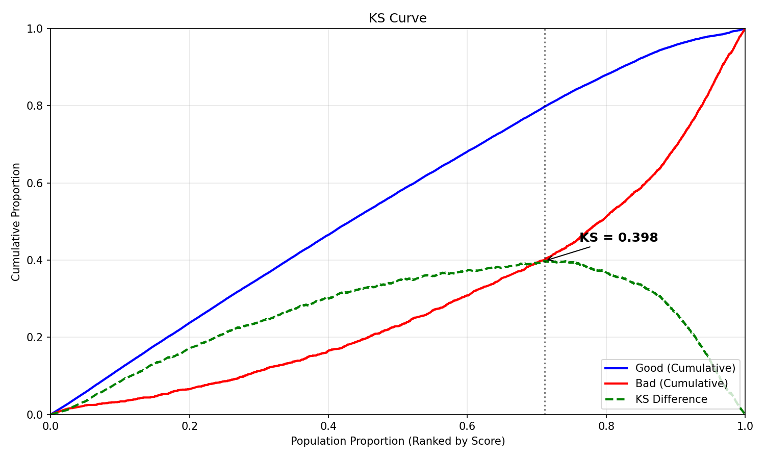
KS: 0.398

Export scorecard table:

from ScoreCardModel.score_card.transformers import ScoreCardTransformer

lr = pipeline.named_steps['model']
bt = pipeline.named_steps['binning']
wt = pipeline.named_steps['woe']
sct = ScoreCardTransformer(lr, bt, wt)
card = sct.export_scorecard()
print(card.head(10))

Output:

 Variable                  Bin       WOE  Points
    PAY_3          (-1.0, 0.0]  0.304362   62.04
    PAY_3         (-inf, -1.0]  0.353610   62.67
    PAY_3           (0.0, inf] -1.393825   40.22
LIMIT_BAL      (-inf, 50000.0] -0.520152   51.85
LIMIT_BAL (100000.0, 180000.0]  0.159326   60.05
LIMIT_BAL (180000.0, 270000.0]  0.301749   61.77
LIMIT_BAL      (270000.0, inf]  0.589377   65.24
LIMIT_BAL  (50000.0, 100000.0] -0.165176   56.13
 PAY_AMT1        (-inf, 316.0] -0.638325   52.43
 PAY_AMT1     (1714.0, 3000.0]  0.042485   58.50

Visualizations

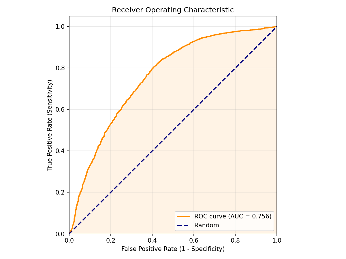
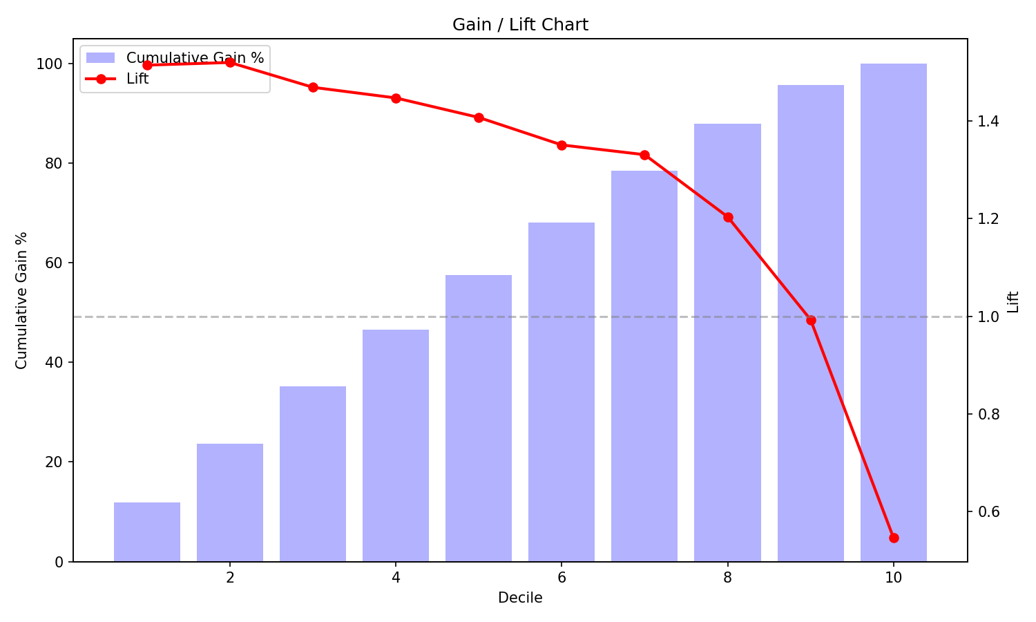
All plots are generated from a model trained on the Taiwan Credit dataset with 9 features selected via rank_features() + select_by_correlation(). The plots below are real output — not mockups.

Model Discrimination

KS Curve	ROC Curve	CAP Curve

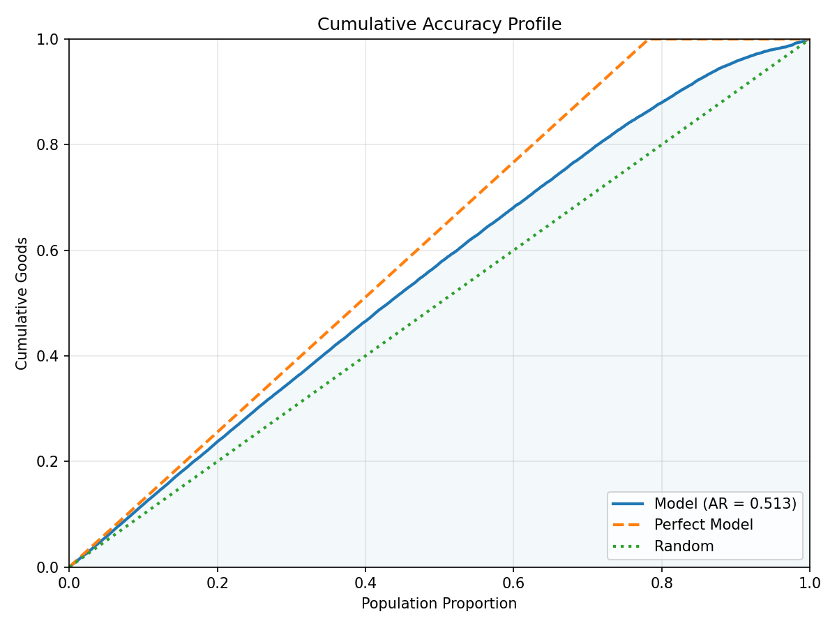KS measures the maximum separation between good and bad populations. ROC shows the trade-off between TPR and FPR. CAP (Cumulative Accuracy Profile) shows the model's cumulative lift over random selection.

Performance Diagnostics

Gain / Lift	Score Distribution	Calibration

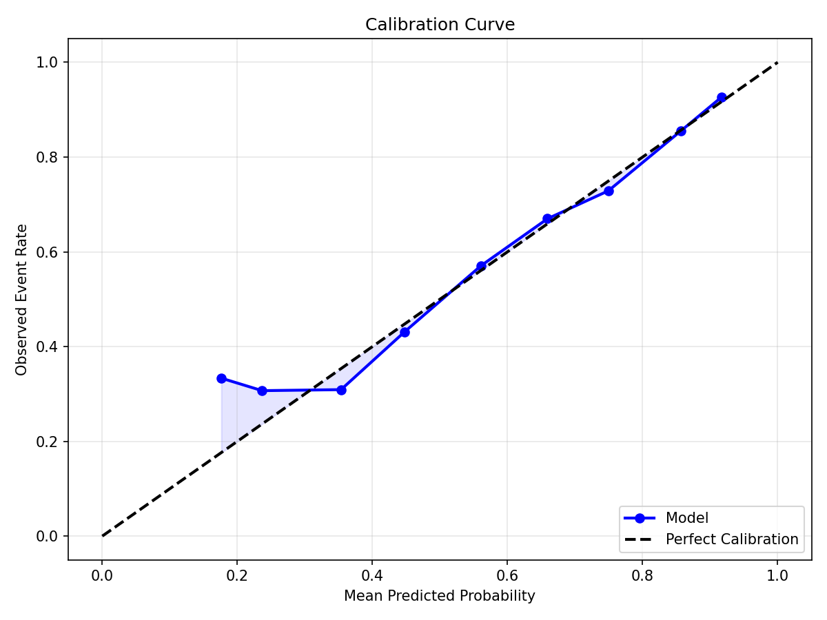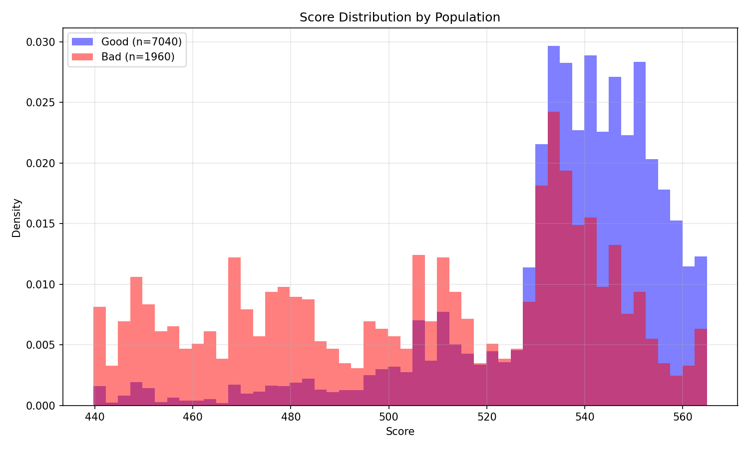
Gain/Lift charts show how well the model ranks risk at each decile. Score distribution compares score profiles of good vs bad accounts. Calibration plots assess whether predicted probabilities match observed event rates.

WOE and IV Analysis

WOE Pattern	IV Summary

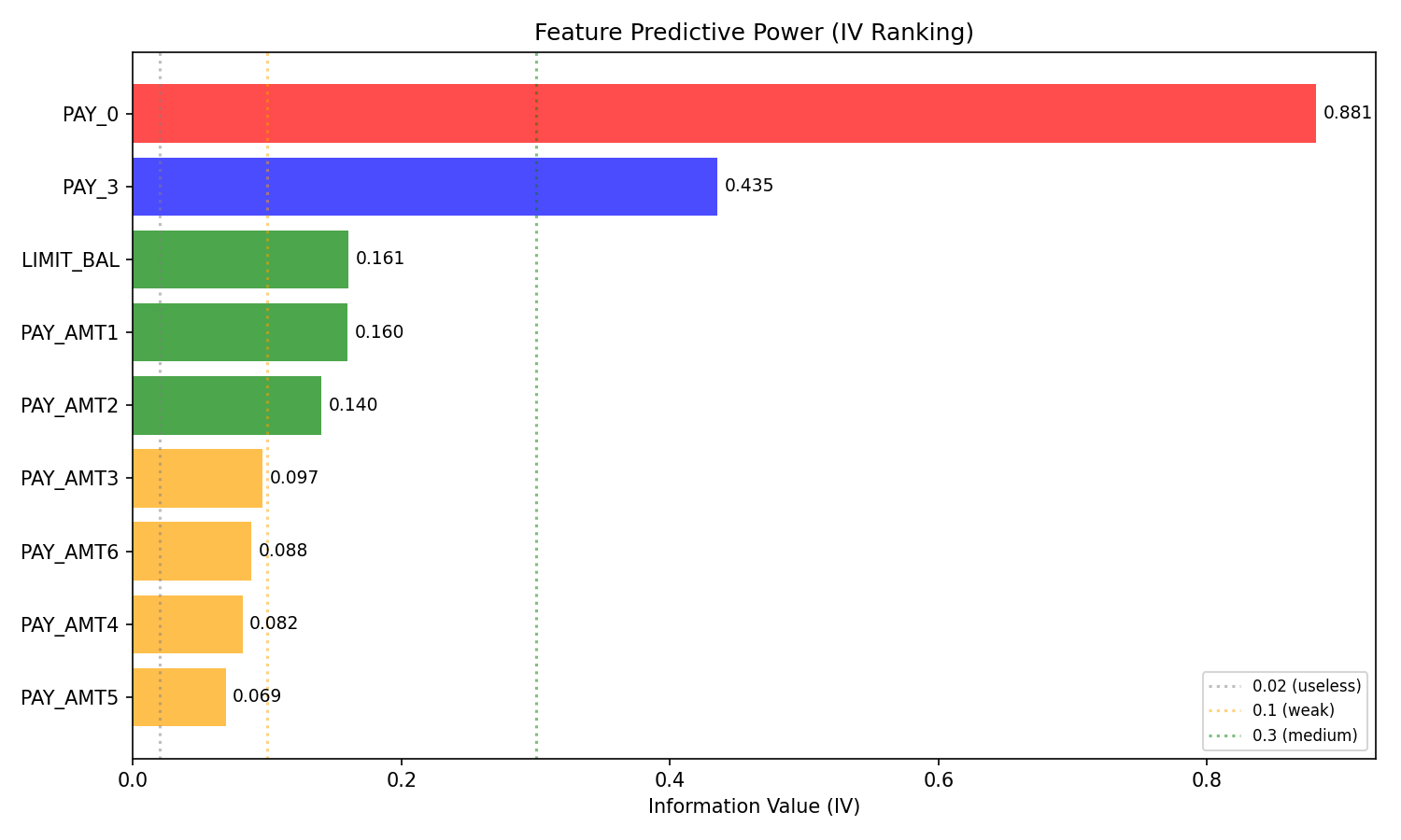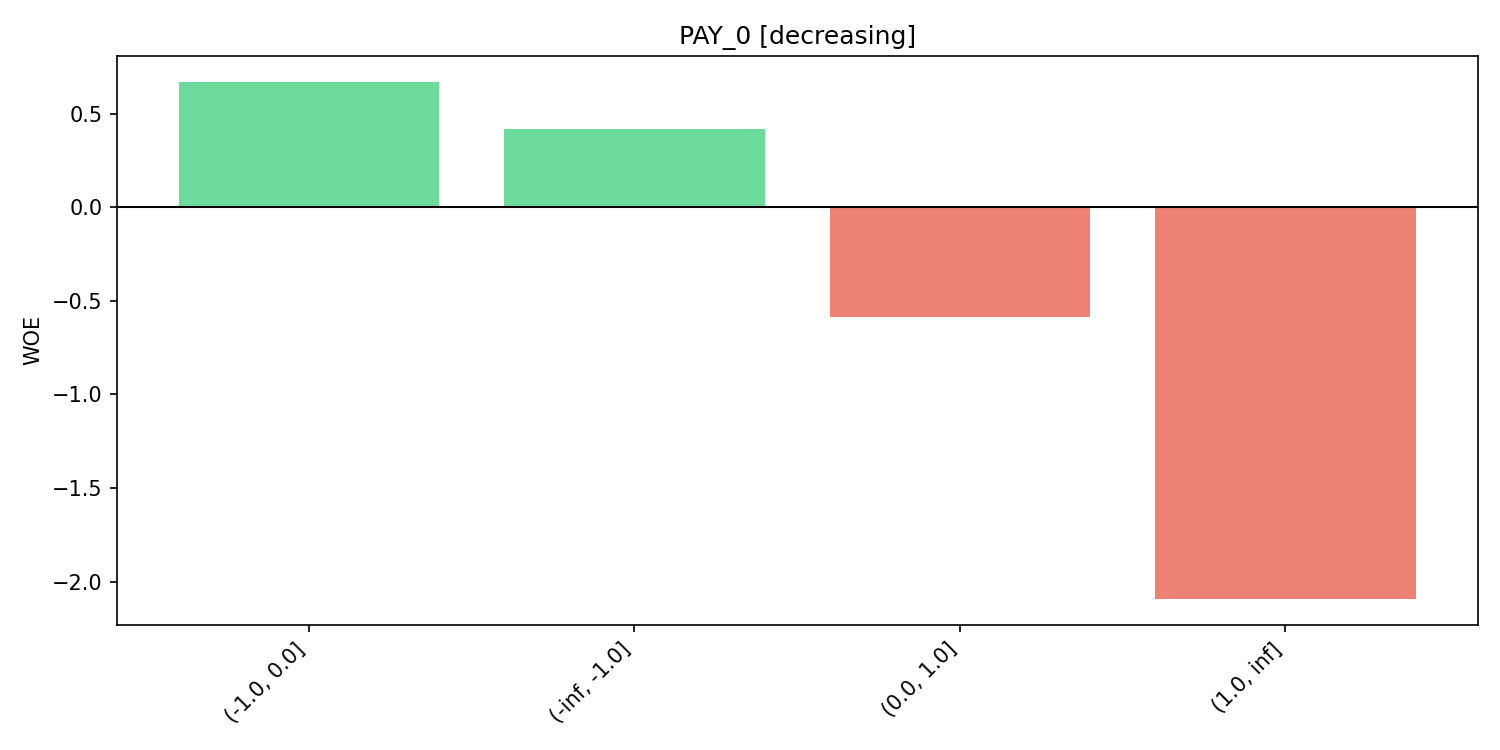
WOE pattern plots show the relationship between bins and their Weight of Evidence. IV summary ranks features by Information Value for feature selection.

Scorecard Interpretation

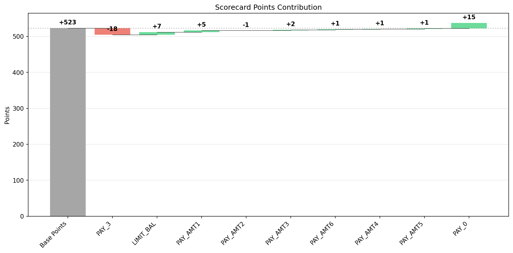
Scorecard Waterfall	Scorecard Heatmap

Waterfall charts show how each feature contributes to the final score. Heatmaps provide a bird's-eye view of the scorecard table.

Decision Threshold

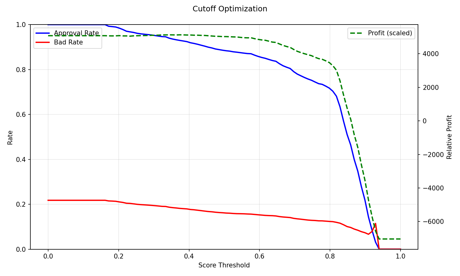
Cutoff Optimization	Confusion Matrix

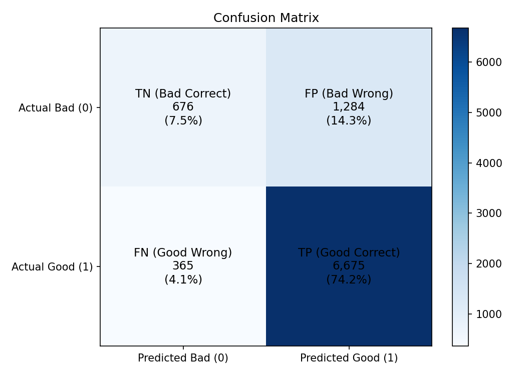Cutoff optimization identifies the optimal decision threshold by balancing cost/benefit. The confusion matrix shows classification performance at the chosen cutoff.

Automated Report

from ScoreCardModel.analytics.reporting import generate_report

generate_report(pipeline, X_train, y_train, X_test, y_test,
                output_path="scorecard_report.md")

The report is a markdown file with embedded PNG plots and the full scorecard table — suitable for sharing with stakeholders or regulatory review.

View Taiwan Credit Report

# Requires: pip install scorecard-toolkit[interactive]
from ScoreCardModel.interactive import ScorecardWidget

widget = ScorecardWidget(pipeline, X_train)
widget.display()

Opens an interactive dashboard in the notebook: sliders/dropdowns for each feature, real-time score display, and a live waterfall chart. The widget is purely client-side — no server needed.

View Interactive Notebook

Dataset Examples

The following examples demonstrate the full scorecard workflow on four real-world datasets spanning different domains, sizes, and data types.

German Credit

1,000 rows, 20 features (7 numeric + 13 categorical)
30% default rate
Demonstrates mixed-type handling — categorical features are auto-detected by BinningTransformer
Full report includes score distribution, KS curve, ROC, scorecard table, and cutoff analysis

data = fetch_openml('credit-g', as_frame=True, parser='pandas')
X, y = data.data, (data.target == 'good').astype(int)

ranking = rank_features(X_train, y_train, n_bins=4)
final = ranking[ranking['Recommendation'].isin(['Accept', 'Investigate'])]['Feature'].tolist()
# 13 features selected

KS: 0.481

View Report

Taiwan Credit (Default of Credit Card Clients)

30,000 rows, 23 numeric features
22% default rate
Features renamed from x1–x23 to UCI names (PAY_0–PAY_6 = payment status, LIMIT_BAL = credit limit, PAY_AMT1–PAY_AMT6 = payment amounts, etc.)
Demonstrates large-dataset performance with 9 selected features (after correlation filter)

data = fetch_openml('default-of-credit-card-clients', as_frame=True, parser='pandas', version=1)
X = data.data.rename(columns=COLUMN_MAP)
y = (data.target == '0').astype(int)

ranking = rank_features(X_train, y_train, n_bins=5)
final = select_by_correlation(X_train[candidates], max_corr=0.7)
# 9 features: PAY_0, PAY_3, LIMIT_BAL, PAY_AMT1–PAY_AMT6

KS: 0.398

View Report

Give Me Some Credit

150,000 rows, 10 features (6 integer + 4 float)
6.7% default rate — heavily imbalanced
Requires missing value imputation for MonthlyIncome (20% NaN) and NumberOfDependents (2.6% NaN)
Demonstrates imbalanced dataset handling with 6 selected features

data = fetch_openml('give-me-some-credit', as_frame=True, parser='pandas', version=1)
X, y = data.data, (data.target == '0').astype(int)

X['MonthlyIncome'] = X['MonthlyIncome'].fillna(X['MonthlyIncome'].median())
X['NumberOfDependents'] = X['NumberOfDependents'].fillna(0)

ranking = rank_features(X_train, y_train, n_bins=10)
final = accept + investigate  # 6 features

KS: 0.368

View Report

WOE Method Comparison

The library provides 5 WOE methods. Each transforms bin counts into Weight of Evidence differently. The table below compares their performance on the Breast Cancer dataset:

## WOE Method Comparison (5 bins)

| Method          |     KS |    AUC |   Total IV |
|:----------------|-------:|-------:|-----------:|
| standard        | 0.9841 | 0.9975 |    52.5544 |
| adjusted        | 0.9683 | 0.9974 |   115.201  |
| empirical_logit | 0.9841 | 0.999  |    67.7484 |
| signed          | 0.9841 | 0.9975 |    52.5544 |
| weighted        | 0.9497 | 0.9979 |    10.5295 |

Key observations: - standard — raw ln(dist_good/dist_bad). Highest discriminatory power but can produce ±inf for zero-count bins (handled internally by replacing with 0). - adjusted — default method. Laplace smoothing (1e-6) prevents log(0) with negligible bias. Recommended for most use cases. - empirical_logit — Agresti correction (+0.5). Standard in SAS-based scorecard development. Robust for small bin counts. - signed — symmetric around zero using ln(max/min). Useful when direction matters more than magnitude. - weighted — downweights small bins by population share. Produces lower total IV but can be more stable with uneven bin sizes.

All 5 methods converge on similar KS/AUC when bins are well-populated. Differences emerge with sparse data, extreme class imbalance, or very small bin counts.

# Try different WOE methods
for method in ['standard', 'adjusted', 'empirical_logit', 'signed', 'weighted']:
    pipeline = Pipeline([
        ('binning', BinningTransformer(n_bins=5)),
        ('woe', WOETransformer(method=method)),
        ('model', LogisticRegression(C=1.0)),
    ])
    pipeline.fit(X_train, y_train)
    y_prob = pipeline.predict_proba(X_test)[:, 1]
    print(f"{method:16s} KS={calculate_ks(y_test, y_prob):.4f}")

View WOE In-Depth Guide | Run Comparison Script

Examples

Feature Selection (Step-by-Step)

End-to-End Pipeline

Visualizations

Model Discrimination

Performance Diagnostics

WOE and IV Analysis

Scorecard Interpretation

Decision Threshold

Automated Report

Interactive What-If Widget (Jupyter)

Dataset Examples

German Credit

Taiwan Credit (Default of Credit Card Clients)

Give Me Some Credit

WOE Method Comparison