Scorecard Model Report
Executive Summary
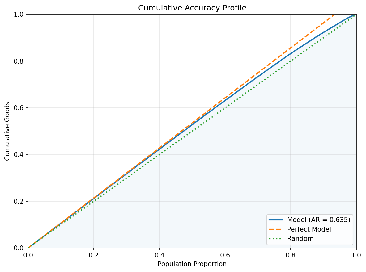
This report evaluates a credit scorecard model built on 7 features using Logistic Regression with adjusted WOE transformation. The model achieves a KS statistic of 50.4% and an AUC of 0.817 (Accuracy Ratio = 0.635), indicating strong discriminatory power between good and bad accounts.
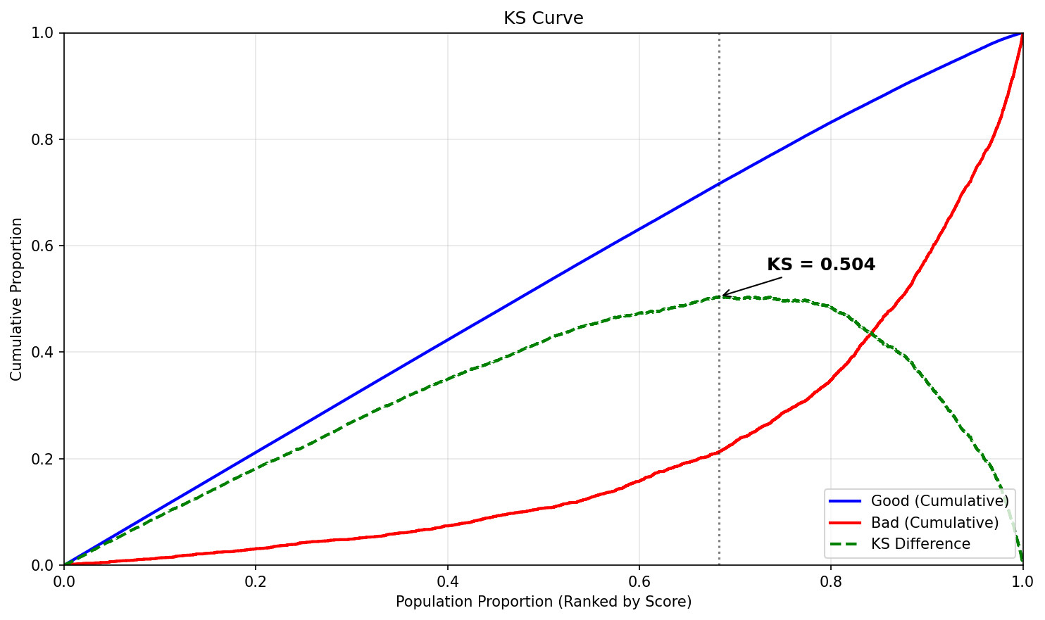
KS = 50.4% — the maximum separation between cumulative good and bad distributions. This is considered strong (good) for credit scorecards.
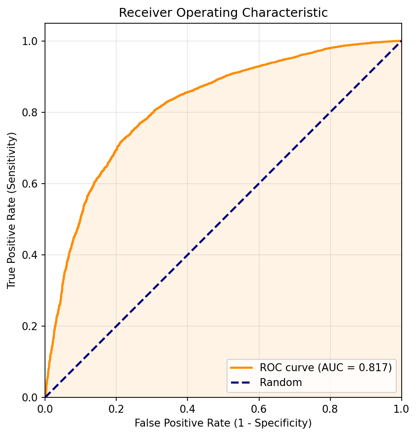
AUC = 0.817 — the probability that the model ranks a randomly chosen good account higher than a randomly chosen bad account. An AUC of 0.5 is random; values above 0.9 are excellent.
Model Performance
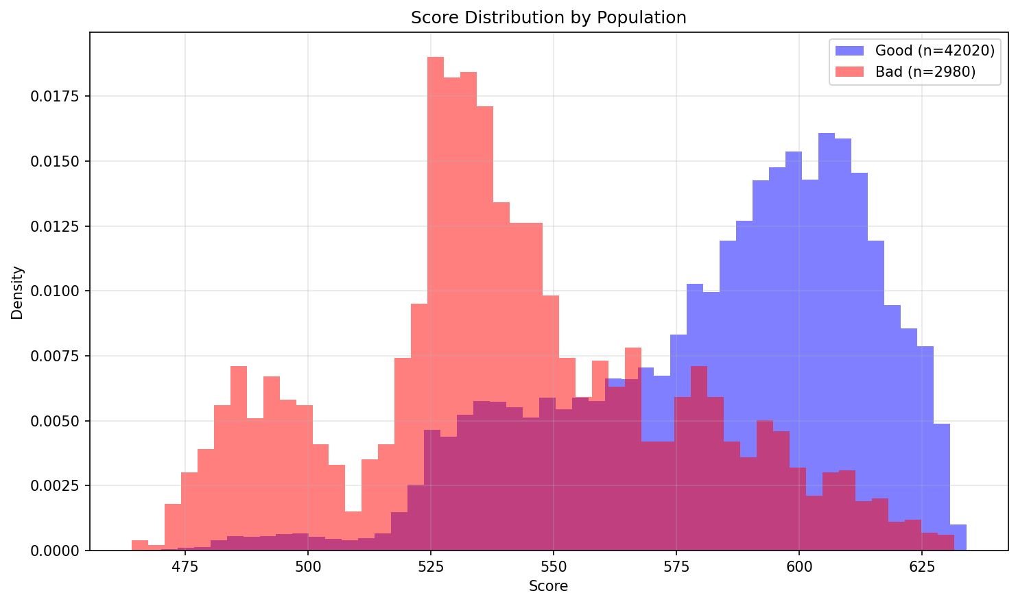
The four plots below assess the model's ability to separate good from bad accounts across the entire score range.
Score Distribution: Good vs Bad
Overlaid density of scores for good (blue) vs bad (red) accounts. Good separation means the two distributions have minimal overlap.
KS Curve
Cumulative proportion of goods and bads as we move from high-risk to low-risk scores. The KS statistic is the maximum vertical distance between the two curves.
ROC Curve
Trade-off between True Positive Rate (sensitivity) and False Positive Rate (1 - specificity). The diagonal line represents a random model.
Cumulative Accuracy Profile (CAP)
Cumulative goods captured as a function of the population fraction, ordered by risk score. The Accuracy Ratio (AR) measures how far the model is from random toward perfect.
Feature Analysis
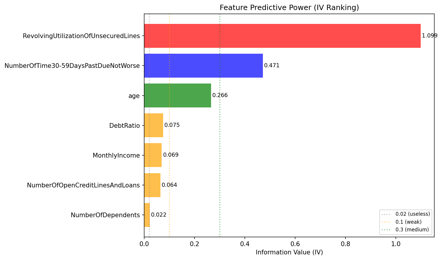
Information Value (IV) measures each feature's predictive power. Industry-standard interpretation: <0.02 useless, 0.02–0.1 weak, 0.1–0.3 medium, 0.3–0.5 strong, >0.5 suspicious (investigate for data leakage).
The model uses 7 features with a total IV of 2.07. The chart below ranks features by individual IV contribution.
Feature IV Ranking
Top Features by IV
The table below ranks the top 10 features. Note the Trend Advice: features with 'Strong Trend (Minor Violations)' are highly predictive but have minor non-monotonic bins. In many practical cases, keeping these features provides significant performance gains compared to enforcing strict monotonicity.
| Feature | IV | Monotonicity | Trend_Advice | Recommendation |
|---|---|---|---|---|
| RevolvingUtilizationOfUnsecuredLines | 1.0987 | non-monotonic | Strong Trend (Minor Violations) | Investigate |
| NumberOfTime30-59DaysPastDueNotWorse | 0.4713 | single_bin | Good | Accept |
| age | 0.2658 | increasing | Good | Accept |
| DebtRatio | 0.0747 | non-monotonic | Irregular | Review (Unstable Trend) |
| MonthlyIncome | 0.0694 | non-monotonic | Irregular | Review (Unstable Trend) |
| NumberOfOpenCreditLinesAndLoans | 0.0644 | non-monotonic | Irregular | Review (Unstable Trend) |
| NumberOfDependents | 0.0222 | decreasing | Good | Accept |
Scorecard
The scorecard translates model log-odds into interpretable point values. Each feature is binned, and each bin is assigned a WOE (Weight of Evidence) and a Points value. Higher points indicate lower risk (more "good"-like). The total score for an applicant is the sum of points across all features plus a base offset.
The table below shows the full scorecard (54 rows across 7 features).
| Variable | Bin | WOE | Points |
|---|---|---|---|
| RevolvingUtilizationOfUnsecuredLines | (-inf, 0.00296] | 1.0218 | 104.74 |
| RevolvingUtilizationOfUnsecuredLines | (0.00296, 0.0192] | 1.58863 | 118.22 |
| RevolvingUtilizationOfUnsecuredLines | (0.0192, 0.0435] | 1.64347 | 119.53 |
| RevolvingUtilizationOfUnsecuredLines | (0.0435, 0.0835] | 1.31979 | 111.83 |
| RevolvingUtilizationOfUnsecuredLines | (0.0835, 0.155] | 1.0374 | 105.12 |
| RevolvingUtilizationOfUnsecuredLines | (0.155, 0.272] | 0.652794 | 95.97 |
| RevolvingUtilizationOfUnsecuredLines | (0.272, 0.446] | 0.267216 | 86.8 |
| RevolvingUtilizationOfUnsecuredLines | (0.446, 0.699] | -0.298472 | 73.35 |
| RevolvingUtilizationOfUnsecuredLines | (0.699, 0.982] | -1.01642 | 56.28 |
| RevolvingUtilizationOfUnsecuredLines | (0.982, inf] | -1.43178 | 46.41 |
| NumberOfTime30-59DaysPastDueNotWorse | (-inf, 1.0] | 0.259014 | 85.91 |
| NumberOfTime30-59DaysPastDueNotWorse | (1.0, inf] | -1.8901 | 40.58 |
| age | (-inf, 33.0] | -0.597678 | 72.49 |
| age | (33.0, 39.0] | -0.396477 | 75.17 |
| age | (39.0, 44.0] | -0.281406 | 76.7 |
| age | (44.0, 48.0] | -0.202462 | 77.75 |
| age | (48.0, 52.0] | -0.140701 | 78.58 |
| age | (52.0, 56.0] | 0.0228395 | 80.75 |
| age | (56.0, 61.0] | 0.297505 | 84.41 |
| age | (61.0, 65.0] | 0.640892 | 88.99 |
| age | (65.0, 72.0] | 0.966864 | 93.33 |
| age | (72.0, inf] | 1.1912 | 96.32 |
| DebtRatio | (-inf, 0.0311] | 0.251918 | 84.76 |
| DebtRatio | (0.0311, 0.134] | -0.0511857 | 79.58 |
| DebtRatio | (0.134, 0.214] | 0.104401 | 82.23 |
| DebtRatio | (0.214, 0.288] | 0.236828 | 84.5 |
| DebtRatio | (0.288, 0.367] | 0.198154 | 83.84 |
| DebtRatio | (0.367, 0.468] | 0.0100847 | 80.62 |
| DebtRatio | (0.468, 0.649] | -0.278209 | 75.7 |
| DebtRatio | (0.649, 4.0] | -0.56282 | 70.83 |
| DebtRatio | (1262.0, inf] | 0.310298 | 85.75 |
| DebtRatio | (4.0, 1262.0] | 0.0961437 | 82.09 |
| MonthlyIncome | (-inf, 2313.9] | -0.256377 | 78.23 |
| MonthlyIncome | (10733.2, inf] | 0.448797 | 84.33 |
| MonthlyIncome | (2313.9, 3400.0] | -0.388132 | 77.09 |
| MonthlyIncome | (3400.0, 4333.0] | -0.248711 | 78.3 |
| MonthlyIncome | (4333.0, 5375.0] | -0.132815 | 79.3 |
| MonthlyIncome | (5375.0, 5400.0] | 0.188717 | 82.08 |
| MonthlyIncome | (5400.0, 6612.3] | -0.00543607 | 80.4 |
| MonthlyIncome | (6612.3, 8265.0] | 0.220191 | 82.36 |
| MonthlyIncome | (8265.0, 10733.2] | 0.290461 | 82.96 |
| NumberOfOpenCreditLinesAndLoans | (-inf, 3.0] | -0.504387 | 76.91 |
| NumberOfOpenCreditLinesAndLoans | (10.0, 12.0] | 0.108107 | 81.21 |
| NumberOfOpenCreditLinesAndLoans | (12.0, 15.0] | 0.0556667 | 80.84 |
| NumberOfOpenCreditLinesAndLoans | (15.0, inf] | -0.0318867 | 80.23 |
| NumberOfOpenCreditLinesAndLoans | (3.0, 4.0] | 0.0294503 | 80.66 |
| NumberOfOpenCreditLinesAndLoans | (4.0, 5.0] | 0.042937 | 80.75 |
| NumberOfOpenCreditLinesAndLoans | (5.0, 6.0] | 0.231159 | 82.07 |
| NumberOfOpenCreditLinesAndLoans | (6.0, 8.0] | 0.253522 | 82.23 |
| NumberOfOpenCreditLinesAndLoans | (8.0, 9.0] | 0.136208 | 81.41 |
| NumberOfOpenCreditLinesAndLoans | (9.0, 10.0] | 0.0976738 | 81.14 |
| NumberOfDependents | (-inf, 1.0] | 0.0833606 | 80.93 |
| NumberOfDependents | (1.0, 2.0] | -0.206635 | 79.25 |
| NumberOfDependents | (2.0, inf] | -0.324535 | 78.57 |
Scorecard Points Heatmap
The heatmap provides a bird's-eye view of the scorecard. Green cells = higher points (lower risk), red cells = lower points (higher risk). Consistent color gradients within each feature indicate good monotonicity.

Calibration & Cutoff
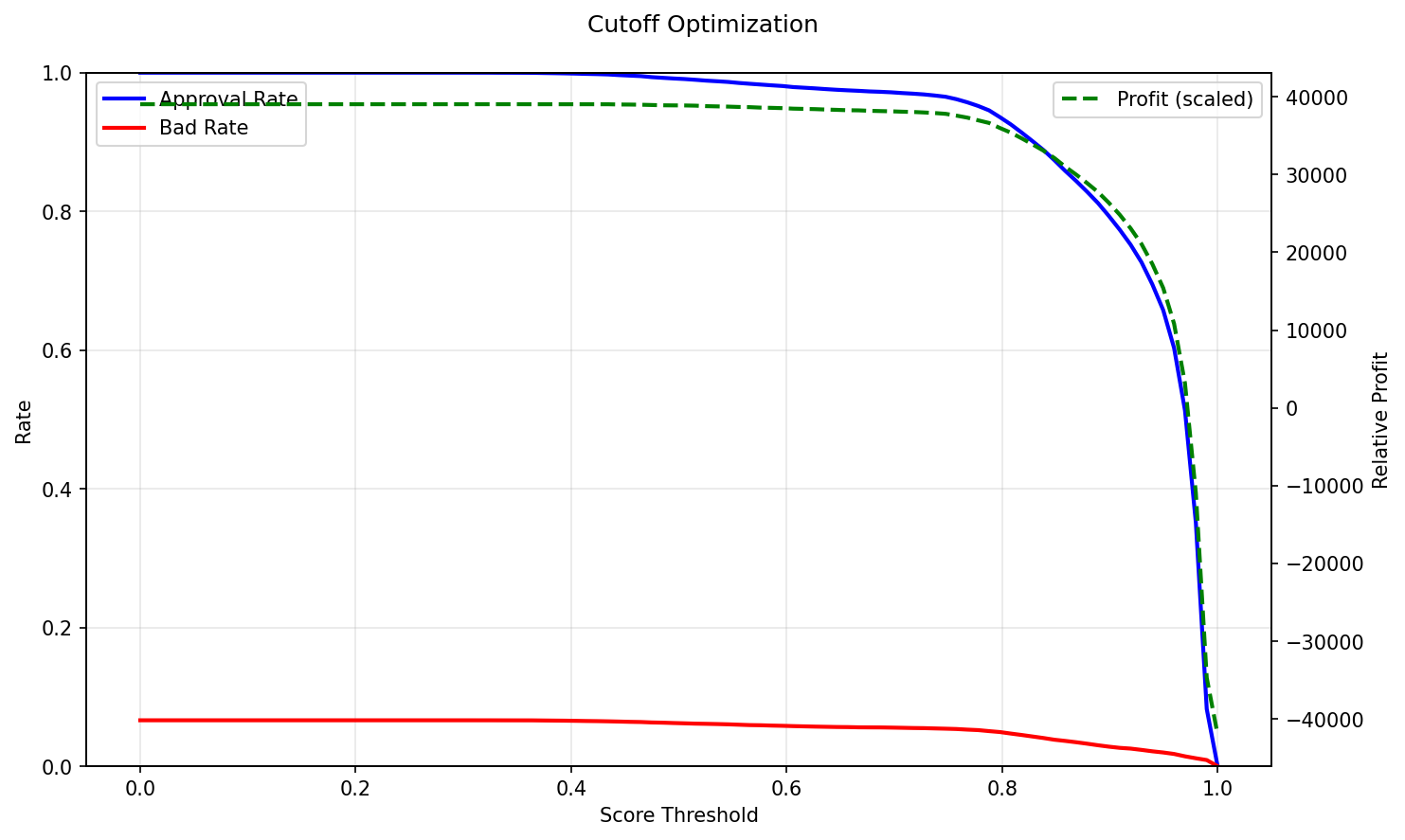
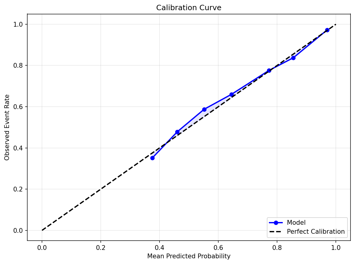
The base event rate in the test set is 93.4%. The plots below assess probability calibration and help select an optimal decision threshold.
Calibration Curve
Compares predicted probabilities against observed event rates. A well-calibrated model follows the diagonal. Points above the line mean the model underestimates risk; below the line means it overestimates.
Cutoff Optimization
Shows how approval rate, bad rate, and relative profit change with the score cutoff. The optimal cutoff balances the cost of false positives (approving a bad account) against false negatives (rejecting a good account).